Statistical examples

One sample, two estimators

The figure shows a one-dimensional generated regression sample, its known mean function, base BNN, and a two-scale estimate. All curves use the same observations. Their differences reveal how locality and signed weights affect the fitted surface.

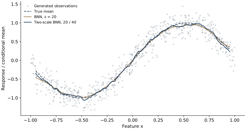
Noisy generated sine regression observations, the true curve, base BNN, and a two-scale BNN fitted curve — Fixed-seed synthetic illustration from examples/figures.py. The generating script records the data, scales, and estimator settings. This is a single realization, not a ranking based on repeated-sample risk.

The explorer supplies a smaller sample whose weights and scale can be inspected directly. Its data and configuration differ from this exported figure.

Separate fit, bias, and uncertainty

At a query x, estimation error is the difference between the fitted value and μ(x). Statistical bias is the expectation of that difference over repeated samples. A curve from one generated dataset displays error; a bias estimate requires repeated sampling or an analytic expectation.

Variance describes how the estimate changes across samples. Bootstrap and jackknife estimate aspects of that sampling variability under their assumptions. Scale selection, feature preprocessing, and the evaluation domain are part of the experiment and should be recorded with the result.

A useful comparison holds the question fixed

Compare estimates at the same queries, on the same samples, for the same estimand. Report error summaries and uncertainty separately. Include the scale-selection rule when it is part of the procedure.

Two-scale correction targets a leading asymptotic bias term. A lower error in every region of every finite sample is a stronger claim than the theory supplies.

One location and a whole region

Pointwise error examines one fixed query. Uniform error takes the largest discrepancy over an evaluation region. A small error at a selected location can coexist with a substantial discrepancy elsewhere.

Pointwise: |μ̂(x₀) − μ(x₀)|
Uniform: sup_{x ∈ K} |μ̂(x) − μ(x)|.

A finite-grid experiment approximates the second object by the maximum on its grid. The spacing, boundaries, and oscillation between grid points matter; a finite grid by itself does not establish a continuum theorem.

Confidence intervals at individual locations and a confidence band covering the entire function are also different inferential objects. The uniform inference discussion explains that distinction.

Reproduce and investigate

git clone https://github.com/jingbowa/bnn.git
cd bnn
python -m pip install '.[benchmark]'
python examples/figures.py

The repository contains the example scripts, independent numerical tests, and paper simulation materials. Saved paper results retain their source manifest; this figure does not rerun the full JASA simulation study.

For a new simulation, record the generating function, feature distribution, noise, sample sizes, dimensions, scales, repetitions, queries, and coverage target. Generate larger experiments on a compute host and publish the script with the result.